A Tutorial on Information Maximizing Variational Autoencoders (InfoVAE)

This tutorial discusses MMD variational autoencoders (MMD-VAE in short), a member of the InfoVAE family. It is an alternative to traditional variational autoencoders that is fast to train, stable, easy to implement, and leads to improved unsupervised feature learning.

Warm-up: Variational Autoencoding

We begin with an exposition of Variational Autoencoders (VAE in short [1,2]) from the perspective of unsupervised representation learning.

Suppose we have a collection of images, and would like to learn useful features such as object categories and other semantically meaningful attributes. However, without explicit labels or the specification of a relevant task to solve, it is unclear what constitutes a “good feature”.

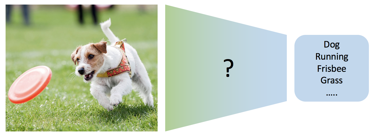
One possibility is to define “good features” as features that are useful for compressing the data. Consider the following setting. Alice is leaving for a space exploration mission. She has a camera that can capture images with 1 million pixels. She would like to send back images to Bob (on Earth), but she can only send 100 bits of information for each image. She has to discuss a communication protocol with Bob before leaving, so that Bob can reconstruct the images as “accurately” as possible with the (short) messages he is going to receive. Luckily, they have an idea of the kind of images \(x \sim p_{\mathrm{data}}(x)\) Alice is going to see based on dataset of images collected by previous space travelers.

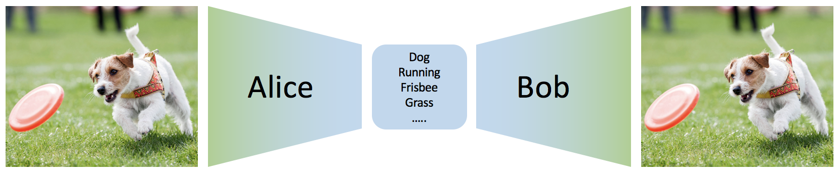
Let \(z\) be the 100 bit message Alice sends (which we term “latent feature”) and \(x\) be image in pixel space. To define a communication protocol, Alice needs to specify an encoding distribution \(q_\phi(z \vert x)\) and Bob a decoding distribution \(p_\theta(x \vert z)\). Here we consider the most general case where encoding and decoding can be randomized procedures. Communication proceeds as follows:

1. Alice observes an image \(x\);
2. Alice produces a distribution over messages, samples ones, and sends to Bob;
3. Bob produces a distribution over possible reconstructions based on the received message, and samples one.

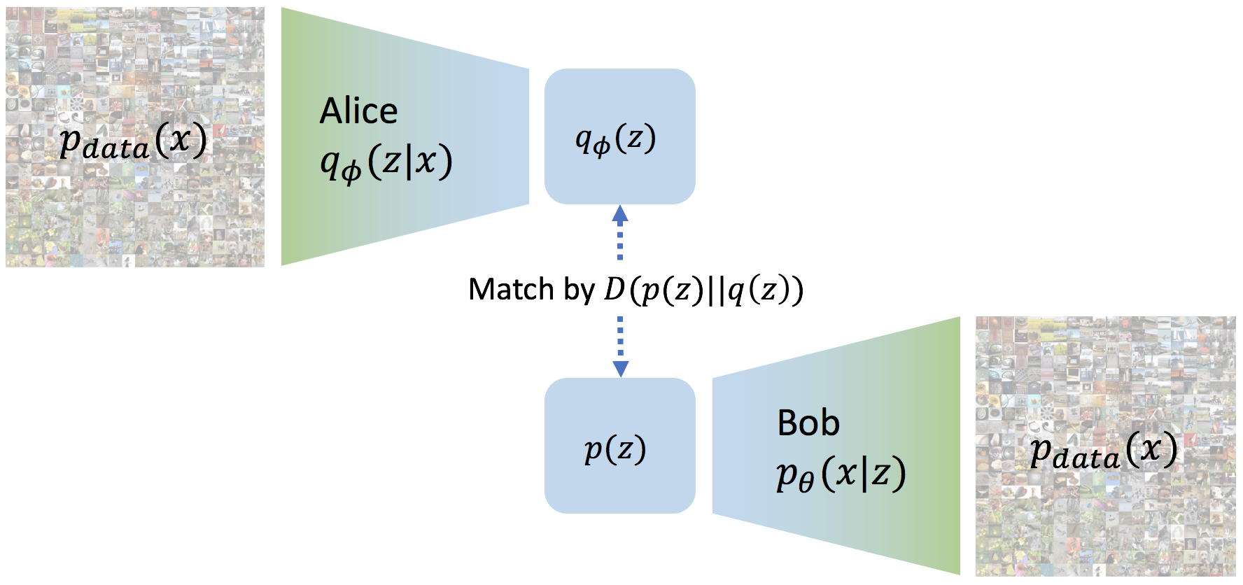
In practice, encoding and decoding distributions are often modeled by deep neural networks, where \(\phi\) and \(\theta\) are the parameters of the neural net.

What remains to be formalized is what we mean by “accurate” reconstruction. This is actually an important open question [3,4], but here we assume that accurate means that the original image Alice wants to send is assigned high probability \(p_\theta(x \vert z)\) by Bob, conditioned on the received message (latent feature \(z\)).

How should we choose the encoding and decoding distributions \(q_\phi\) and \(p_\theta\)? One possibility is to jointly optimize the following reconstruction loss for each image \(x\):

This objective encourages Alice to generate good messages, so that based on the message, Bob assigns high probability to the original image. The hope is that if Alice and Bob can accomplish this, the message (latent feature) should contain the most salient features and capture the main factors of variation in the data.

In addition to this, we may want to enforce additional structure on the message space. For example, Alice should be able to observe an image, generate latent features, change only a part of it (such as certain attributes), and Bob should still be able to generate sensible outputs reflecting the change. It would also be nice for Alice to be able to directly generate valid messages without having to observe actual images.

To do this we must define the space of valid messages. This can be achieved by defining a “prior” distribution of valid messages \(p(z)\). \(p(z)\) is usually a very simple distribution such as a uniform or Gaussian distribution. Accounting for all possible images from the true underlying distribution \(p_{data}(x)\), we get a distribution over possible messages Alice generates \(q_\phi(z) = \mathbb{E}_{p_{data}(x)} [q_\phi(z\vert x)]\). We would like the message distribution Alice generates to match the distribution on valid messages \(p(z)\).

We thus get a general family of variational auto-encoding objectives

where \(D\) is any strict divergence, meaning that \(D(q \Vert p) \geq 0\) and \(D(q \Vert p) = 0\) if and only if \(q = p\), and \(\lambda>0\) is a scaling coefficient.

Which divergence should one choose? The original VAE objective [1] uses \(\mathbb{E}_{p_{data}(x)}[ -\mathrm{KL}(q_\phi(z \vert x) \Vert p(z)) ]\), which is minimized if the message \(q_\phi(z\vert x)\) Alice generates for each input \(x\) matches the prior \(p(z)\). Of course, this implies that the distributions also match when “averaging” over all possible inputs. This can be problematic in some scenarios. For example, it is not clear why we would want Alice to generate the same message for each possible input, as this works against our goal of learning good features. We will return to this crucial aspect later. For now, we introduce an alternative divergence called Maximum Mean Discrepancy [5], which we will show has many advantages compared to traditional approaches.

Maximum Mean Discrepancy

Maximum mean discrepancy (MMD, [5]) is based on the idea that two distributions are identical if and only if all their moments are the same. Therefore, we can define a divergence by measuring how “different” the moments of two distributions \(p(z)\) and \(q(z)\) are. MMD can accomplish this efficiently via the kernel embedding trick:

where \(k(z, z')\) is any universal kernel, such as Gaussian \(k(z, z') = e^{-\frac{\lVert z - z' \rVert^2}{2\sigma^2}}\). A kernel can be intuitively interpreted as a function that measures the “similarity” of two samples. It has a large value when two samples are similar, and small when they are different. For example, the Gaussian kernel considers points that are close in Euclidean space to be “similar”. A rough intuition of MMD, then, is that if two distributions are identical, then the average “similarity” between samples from each distribution, should be identical to the average “similarity” between mixed samples from both distributions.

Why Use an MMD Variational Autoencoder

In this section we argue in detail why we might prefer MMD-VAE over the traditional evidence lower bound (ELBO) criterion used in VAEs:

We show that ELBO suffers from two problems that MMD-VAE

does not suffer from.

Problem 1: Uninformative Latent Code

Researchers have noticed that the term

might be too restrictive [6,7,8]. Intuitively it encourages the message \(q_\phi(z \vert x)\) to be a random sample from \(p(z)\) for each \(x\), making the message uninformative about the input. If the decoder is very flexible, then a trivial strategy can globally maximize ELBO: Alice only produces \(p(z)\) regardless of the input, and Bob only produces \(p_{data}(x)\) regardless of Alice’s message. This means that we have failed to learn any meaningful latent representation. Even when Bob cannot generate a complex distribution (e.g. \(p_\theta(x \vert z)\) is a Gaussian), this still encourages the model to under-utilize the latent code. Several methods have been proposed [6,7,8] to alleviate this problem, but they involve additional overhead, and do not completely solve the issue.

MMD Variational Autoencoders do not suffer from this problem. As shown in our paper, it always prefers to maximize mutual information between \(x\) and \(z\). Intuitively, the reason is that the distribution over messages has to match the prior only in expectation, rather than for every input.

Problem 2: Variance Over-estimation in Feature Space

Another problem with ELBO-VAE is that it tends to over-fit data, and as a result of the over-fitting, learn a \(q_\phi(z)\) that has variance tending to infinity. As a simple example, consider training ELBO on a dataset with two data points \(\lbrace -1, 1 \rbrace\), and both encoder \(q_\phi(z\vert x)\) and decoder \(p_\theta(x\vert z)\) output Gaussian distributions with non-zero variance. We prove in our paper that \(\mathcal{L}_{ELBO}\) can be maximized to infinity by

1. The mean of \(q_\phi(z \vert x=-1)\) tends to \(-\infty\), and the mean of \(q_\phi(z \vert x=1)\) tends to \(+\infty\).
2. The probability density of \(p_\theta(x \vert z<0)\) is concentrated around \(x=-1\), and \(p_\theta(x\vert z>0)\) is concentrated around \(x=1\).

The problem here is that, for ELBO, the regularization term \(\mathrm{KL}(q_\phi(z\vert x) \Vert p(z))\) is not strong enough compared to the reconstruction loss. Instead of forcing \(q_\phi(z) = \frac{1}{2}q_\phi(z \vert x=-1) + \frac{1}{2}q_\phi(z \vert x=1)\) to match \(p(z)\), it prefers to have two modes that are pushed infinitely far from each other. Intuitively, pushing the modes as far as possible from each other reduces ambiguity during reconstruction (the messages corresponding to the two inputs are clearly separated, hence Bob’s decoding is easy). Although there is a preference to match the prior, the reconstruction term in the ELBO objective dominates. This can be experimentally verified and visualized: observe how mass of \(q_\phi(z \vert x)\) is pushed away from \(0\) (top animation) as the model overfits this small dataset (bottom animation).

We cannot simply add a large coefficient \(\beta\) to \(\mathrm{KL}(q_\phi(z \vert x) \Vert p(z))\). Even though adding a coefficient \(\beta\) larger than 1 has been shown to improve generalization [9], this is exactly the term that encourages the model not to use the latent code (Problem 1). Increasing it will make matters worse for the uninformative latent code problem. On the other hand, with the MMD-VAE objective we can freely increase the weight of the regularization term \(\lambda D(q_\phi(z) \Vert p(z))\), with little negative consequences. As shown below, we get much better behavior when \(\lambda = 500\) in the previous example:

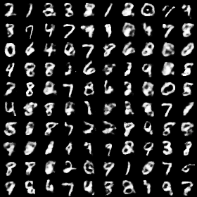
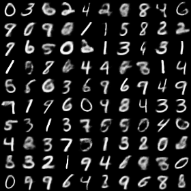
This matters in practice when the dataset is small. For example, when training on MNIST with only 500 examples, ELBO overfits and generates poor samples (Top), while InfoVAE generates reasonable (albeit blurry) samples (Bottom).

Implementing a MMD Variational Autoencoder

The code for this tutorial can be downloaded here, with both python and ipython versions available. The code is fairly simple, and we will only explain the main parts below. (A pytorch version provided by Shubhanshu Mishra is also available.)

To efficiently compute the MMD statistics and exploit GPU parallelism, we use the following code

def compute_kernel(x, y):
    x_size = tf.shape(x)[0]
    y_size = tf.shape(y)[0]
    dim = tf.shape(x)[1]
    tiled_x = tf.tile(tf.reshape(x, tf.stack([x_size, 1, dim])), tf.stack([1, y_size, 1]))
    tiled_y = tf.tile(tf.reshape(y, tf.stack([1, y_size, dim])), tf.stack([x_size, 1, 1]))
    return tf.exp(-tf.reduce_mean(tf.square(tiled_x - tiled_y), axis=2) / tf.cast(dim, tf.float32))

def compute_mmd(x, y, sigma_sqr=1.0):
    x_kernel = compute_kernel(x, x)
    y_kernel = compute_kernel(y, y)
    xy_kernel = compute_kernel(x, y)
    return tf.reduce_mean(x_kernel) + tf.reduce_mean(y_kernel) - 2 * tf.reduce_mean(xy_kernel)

The first function compute_kernel(x, y) takes as input two matrices (x_size, dim) and (y_size, dim), and returns a matrix (x_size, y_size) where the element \((i, j)\) is the outcome of applying the kernel to the \(i\)-th vector of \(x\), and \(j\)-th vector of \(y\). Given this matrix, we can compute the MMD statistics according to the definition. sigma_sqr controls the smoothness of the kernel function, which is a hyper-parameter \(\sigma^2\). We find MMD to be fairly robust to its selection, and that using \(2/dim\) is a good option in our experiments.

To match samples from the prior \(p(z)\) and from the encoding distribution, we can simply generate samples from the prior distribution \(p(z)\), and compare the MMD distance between the real samples and the generated latent codes.

true_samples = tf.random_normal(tf.stack([200, z_dim]))
loss_mmd = compute_mmd(true_samples, train_z)

We suppose that the distribution Bob produces \(p_\theta(x \vert z)\) is a factorized Gaussian. The mean of the Gaussian \(\mu(z)\) is produced by a neural network, and the variance is simply assumed to be some fixed constant. The negative likelihood is thus proportional to the squared distance \(\lVert x - \mu(z) \rVert^2\). The total loss is a sum of this negative log likelihood and the MMD distance.

loss_nll = tf.reduce_mean(tf.square(train_xr - train_x))
loss = loss_nll + loss_mmd

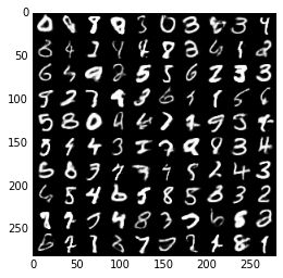
Training on a Titan X for approximately one minute already gives very sensible samples.

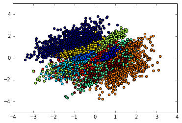
Furthermore if the latent code only has two dimensions, we can visualize the latent code produced by different digit labels. We can observe good disentangling where each color is a digit class.

References

[1] Kingma, Diederik P., and Max Welling. “Auto-encoding variational bayes.” arXiv preprint arXiv:1312.6114 (2013).

[2] Rezende, Danilo Jimenez, Shakir Mohamed, and Daan Wierstra. “Stochastic backpropagation and approximate inference in deep generative models.” In International conference on machine learning, pp. 1278-1286. PMLR, 2014.

[3] Larsen, Anders Boesen Lindbo, Søren Kaae Sønderby, Hugo Larochelle, and Ole Winther. “Autoencoding beyond pixels using a learned similarity metric.” In International conference on machine learning, pp. 1558-1566. PMLR, 2016.

[4] Dosovitskiy, Alexey, and Thomas Brox. “Generating images with perceptual similarity metrics based on deep networks.” Advances in neural information processing systems 29 (2016): 658-666.

[5] Gretton, Arthur, Karsten Borgwardt, Malte Rasch, Bernhard Schölkopf, and Alex Smola. “A kernel method for the two-sample-problem.” Advances in neural information processing systems 19 (2006): 513-520.

[6] Chen, Xi, Diederik P. Kingma, Tim Salimans, Yan Duan, Prafulla Dhariwal, John Schulman, Ilya Sutskever, and Pieter Abbeel. “Variational lossy autoencoder.” arXiv preprint arXiv:1611.02731 (2016).

[7] Bowman, Samuel R., Luke Vilnis, Oriol Vinyals, Andrew M. Dai, Rafal Jozefowicz, and Samy Bengio. “Generating sentences from a continuous space.” arXiv preprint arXiv:1511.06349 (2015).

[8] Sønderby, Casper Kaae, Tapani Raiko, Lars Maaløe, Søren Kaae Sønderby, and Ole Winther. “Ladder variational autoencoders.” Advances in neural information processing systems 29 (2016): 3738-3746.

[9] Higgins, Irina, Loic Matthey, Arka Pal, Christopher Burgess, Xavier Glorot, Matthew Botvinick, Shakir Mohamed, and Alexander Lerchner. “beta-vae: Learning basic visual concepts with a constrained variational framework.” (2016).